results
Because what is the point of doing something without results
gel electrophoresis
The results of the adjusments of buffer, temperature, and annealing time are included in this section.
Experiment 1. The first annealing process was done with temperature steadily decreasing from 91°C to 45°C for 12 hours. MgCl2 was kept at 5mM, 10mM, 15mM, 20mM (lane 2 to 5, respectively). Lane 1 is the DNA marker.
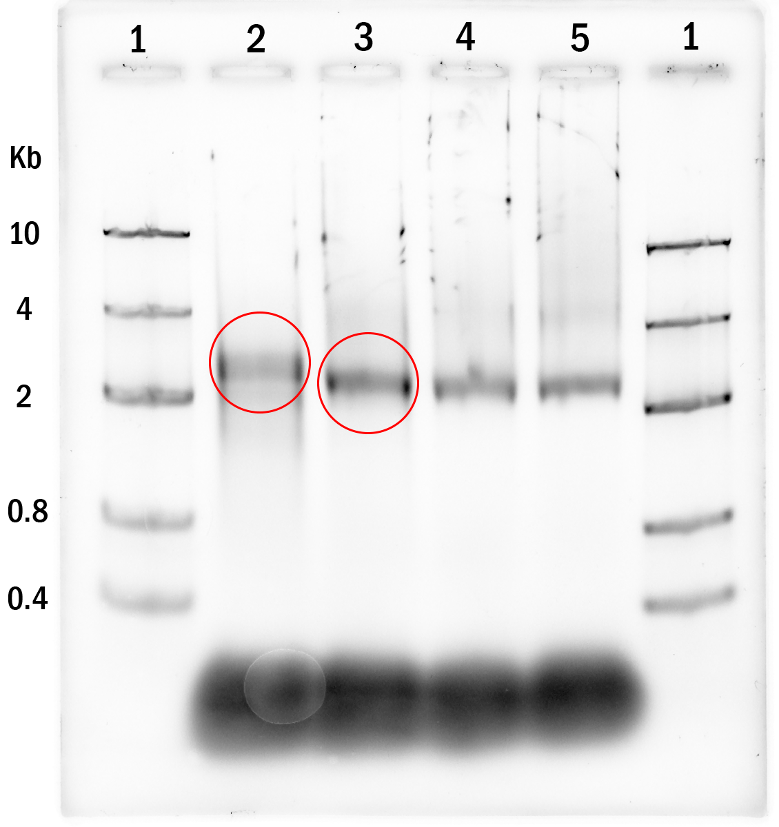
to be brought on to the next experiments.
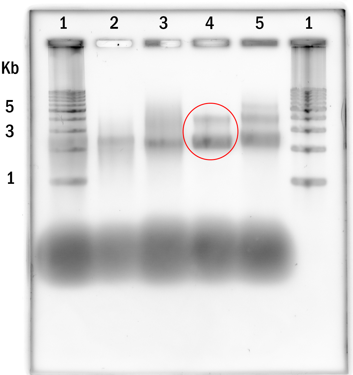
Experiment 2. Variations in temperature, Lane 2-5 were annealed with 10mM MgCl2 and 6-9 were annealed with 20mM MgCl2. Temperature was kept constant for 12 hours at: 52°C, 55°C, 58°C, 59°C, 52°C, 55°C, 58°C, 59°C. (lane 2-9 respectively). Lane 1 is the DNA marker.

55°C and 10mM MgCl2 and were brought on to the next experiments.
Experiment 3. Combination of experiment 2 and 1, the best results from experiments 1 and 2 were further tested to find the ideal concentration of MgCl2 and temperature. All annealing process took 12 hours. The condition was set to: 5mM MgCl2 91-45°C, 10mM MgCl2 91-45°C, 10mM MgCl2 55°C, 10mM MgCl2 65°C (lane 2-5 respectively). Lane 1 is the DNA marker.
concentration was decided to be 55°C and 10mM.
determination of optimal annealing time
As the optimal temperature and MgCl2 concentration for the annealing process was decided from the previous experiments. The time needed for perfect annealing process was then experimented.
Experiment 4. Determination of optimal annealing time was done with 2 hour intervals until 12 hours.
Annealing time was set at: 0h, 2h, 4h, 8h, 12h. (lane 2-6 respectively). Lane 1 is the DNA marker.
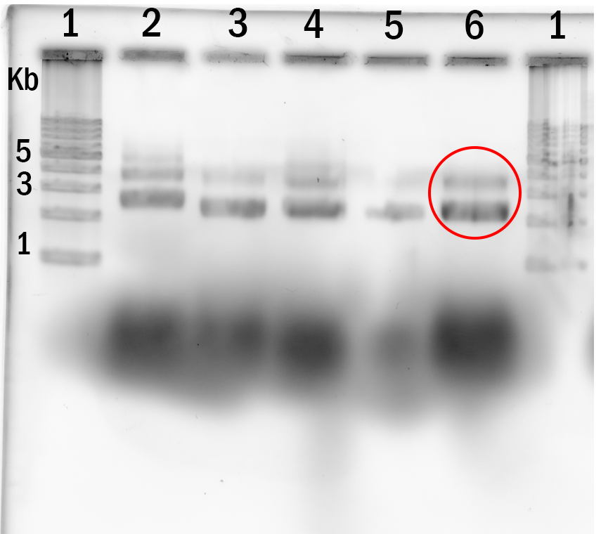
In conclusion we used 55°C and 10mM MgCl2 concentration along with 12h annealing time to produce the structures we needed for the observations.
AFM
Before analysis by FRET, firstly we used our most readily available microscope, AFM which is short for atomic force microscopy. Through AFM observation, we can roughly estimate if the planned structure has formed.
Even though it is a microscope, it is not a conventional microscope that uses source of light to image the object, but it senses the depth of the sample through the interaction of the tip of the microscope and the sample, and that is exactly why it can have better resolutions than conventional light microscopes. The sensor detects the deflection of the laser that is projected into the cantilever tip and thus the movement of the tip of the cantilever can be measured. We expected a length of around 50nm and a diameter/width of about 18nm for the outer tube.

laser and the sensor and thus the depth of the sample is registered.
After deciding the final conditions for the annealing process, observation under AFM was conducted and the following images were taken:
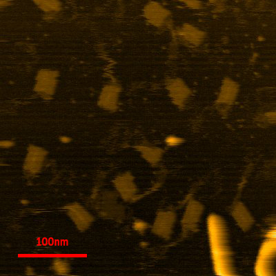
after annealing.
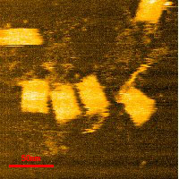
Measurements were taken for the length and the width of the outer tube. The results are as follows:
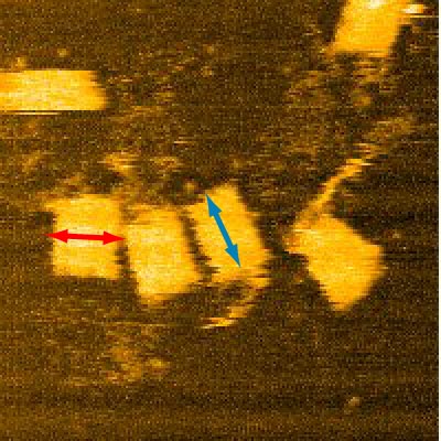
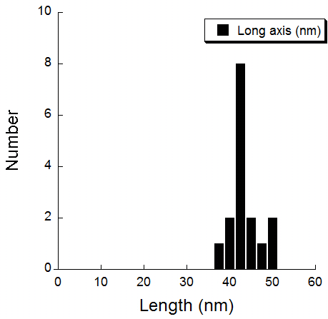
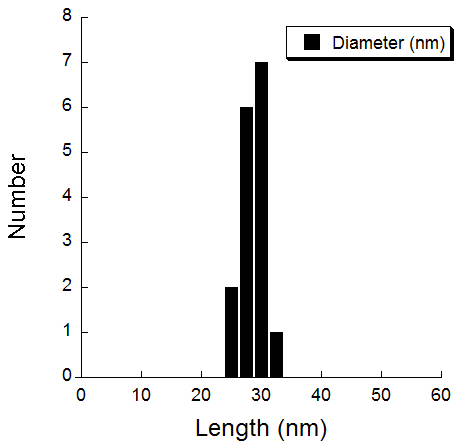
Measurements taken from 16 different structures yielded length of 45+/-3nm and diameter of 30+/-2nm, the tip of AFM might have deformed the structure causing it to be wider, further observations using TEM might be able to clarify this point. Even though the structure was clearly seen through AFM (Tube and loops clearly seen), it is inconclusive without the data of the depth of the structure. Therefore, we measured the depth of 2 selected structures from end to end to understand if our structure had actually folded properly.

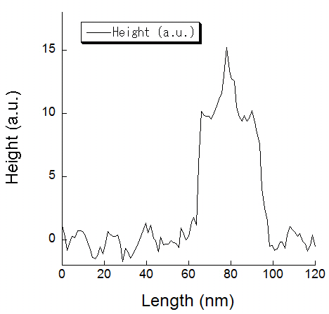
From here we can see that the width is about 40nm.
.jpg)
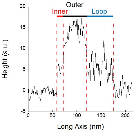
70-120nm denoted the outer tube and finally the loop was shown from around 120-175.
fret
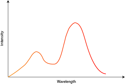
FRET (Fluorescence resonance energy transfer) is used to observe subtle difference in movement of the parts in the structure. It works by having two different fluorophores with different excitation spectra but one has an emission spectrum that corresponds to the other spectrum. The energy transfer occurs at a very close distance (1-10nm) and therefore it can be used to judge the movement of a point in the structure in relation to another.

in this experiment, Cy3 would be the orange line and Cy5 would be the red line
the distance is too far for resonance to occur.
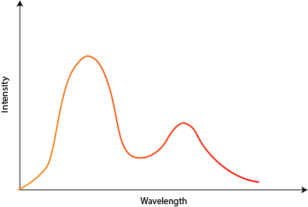

the distance is close enough for resonance to occur.
The fluorophores are attached to two staples, one in the outer tube and one in the inner tube.

Fig 4.20. The approximate positions of the fluorophores. Note that the positions
of the fluorophores are at the end of each tubes to prevent it from hindering the sliding movement.
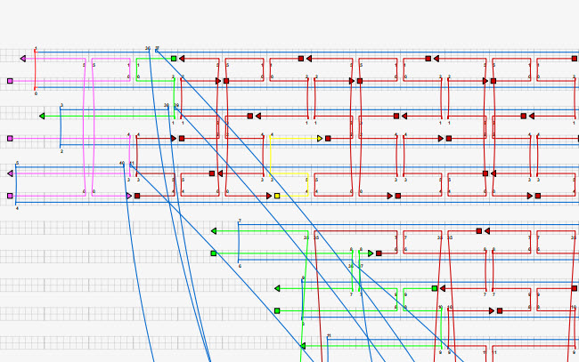

Fig 4.21. and 4.22. The staples seen from cadnano (yellow)
The details of the sequences are as follows:
| Name | Sequence |
|---|---|
| Cy3 | 5’ TTT TAT CCG CGA CCT TGA CAA GAA C 3’ (CY3) |
| Cy5 | 5’ ACT GGA TTA TCA TTT TTC TTT T 3’ (CY5) |
Table 3. Staples modified to accommodate for the fluorophores: Cy3 and Cy5.
The results of the FRET observation are as follows:
of fluorophores, Cy3 (left) and Cy5 (right)
which can be seen alternately emitting
different light spectrum.

from Fig 4.23. showed that the position of the
Cy5 molecules on the right side correspond
to the Cy3 molecules on the left side.
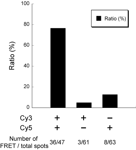
In conclusion, the movement of the outer tube relative to the inner tube was successfully performed and observed. However, it should be noted that in this final confirmation of movement, the main driving force of the movement of the inner tube relative to the outer tube was brownian motion and not through magnet. Nevertheless, the movement was just as expected, as the results shown in 4.23 was conclusive.
Experiment
Now, you might want to ask how are we going to maintain the orientation of our individual structures to enable it to react to a magnet. The solution we proposed was to replace some of the normal DNA staple on the loop edge of the outer tube with biotinylated staple. Then, this end will be able to be fixed on a flat surface coated with peg-biotin through avidin intermediate.
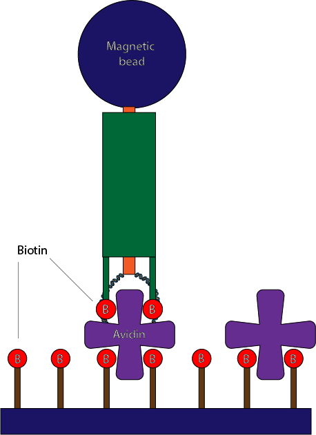
Fig 4.26. Fixation of the molecule on a surface through avidin intermediate.
The sequences of the staples that we changed are as follows:
| Name | Sequence |
|---|---|
| Biotin (192) | Biotin 5’ TT TTT TTT TTT GGT GTA TCA CCG TAC TCA GAA TTT AGG CAG AGG CAT TTT TTT 3’ |
| Biotin (111) | Biotin 5’ TT TTT TTT TTT TTT TTT TAG CAG CAC CGT AAT CAG TAA TTA GCG TTT GCC ATC TTT TTT T 3’ |
| Biotin (133) | Biotin 5’ TT TTT TTT TTT TTT AAG TTT ATT TTG TCA CAA AGA CAC CAC GGA ATT TT 3’ |
| Biotin (193) | Biotin 5’ TT TTG CAG CCT TTA CAG AGA GAA CCA ATA ATA TTT T 3’ |
Table 4. Staples modified with biotin to enable fixation.
As in the previous experiment, the magnetic bead was attached to the inner tube using biotinylated staple, however for them to not intervene with other biotinylated staple, they had to be replaced with DNA staples with a different modifier, in this case amino modifier or the addition of NH2 and a 12 carbon intermediate. In turn, the magnetic bead should be replaced with carboxyl group coated magnetic beads.
Sequences of the staples are as following:
| Name | Sequence |
|---|---|
| NH2 (199) | NH2 (12C) 5’ TA AAA GAA GTT TTT TCC AGA CGT TTT 3’ |
| NH2 (198) | NH2 (12C) 5’ TT TTT TAG TAA ATG AAT TTT GTC GTC TGC CAG AG 3’ |
| NH2 (200) | NH2 (12C) 5’ TT TTT TTT AGA GGC GGT TTG AAT AGC GAG AGG CTT TTG CTT TT 3’ |
Table 5. Staples modified for connection to carboxyl coated magnetic beads.